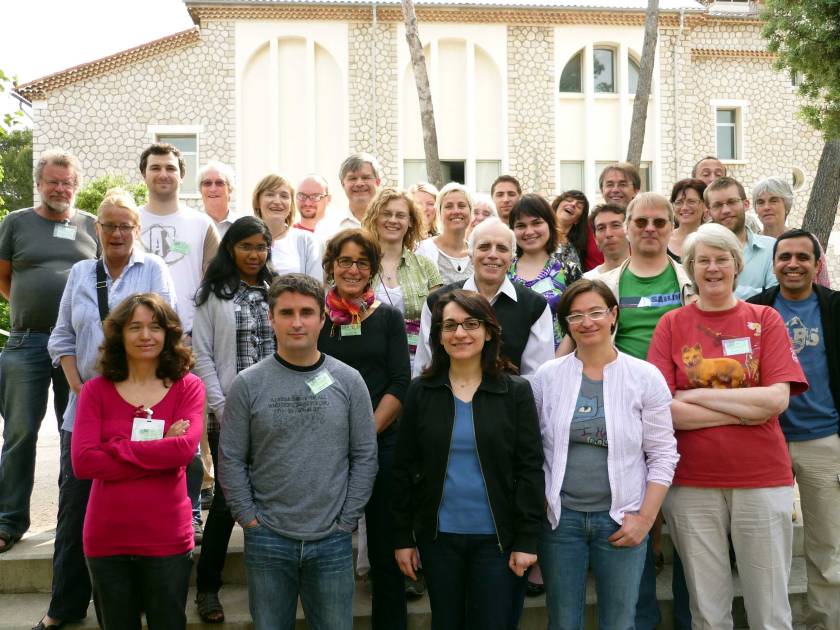
EPD Open Science Meeting and workshops. Prague, 1st-3rd June, 2022.

Latest news, accommodation details and practicals.

We are looking forward to meet you in Prague! Before our meeting, you may find this document useful. In it you will find details about the venue, transport, accommodation, lunches, posters and more! we would like to draw you attention to some final details:

1. For those of you with your accommodation supported by PAGES, you can see your accommodation assignation here. We however advice you to come first to the reception desk on Wednesday 1st at 1pm so we give you all the needed information to get there and will update the room numbers if necessary. In addition, at this welcoming desk we will provide you with a public transport ticket, valid for three days, for you to connect between the conference venue and the accommodation area (ca. 45′ by transport, all details are in the previous section document).

2. We have finalized now the workshop assignation, see here. The Chronology and Tilia workshops will run only once (Thursday and Friday respectively). You will be contacted by the workshop organizer in case anything is required before the conference. Please note that all workshops require you having your own laptop and for most you need to have R and R-Studio installed. If you are interested in following the Tilia workshop note that this is a windows program and can only be installed on a Windows PC or Windows emulator.


3. If you are presenting a poster, remember to prepare one single slide summarizing it and be ready to give a 1minute flash talk of it. You will have to hand out this slide at the welcoming desk on Wednesday the 1st from 1 to 2pm.

4. During the poster session we invite you to bring sweets and snacks or drinks typical from your country of origin to share with the rest of us.

5. Those of you attending the BBQ on Friday, be ready to pay at the welcoming desk (either in CZK or EUR) from 5 to 10€ to cover the food costs – there is not a fixed amount and we leave it to your own appetite 🙂 Drinks can be bought on location.

6. Here you have some additional information regarding where to eat, nightlife and public transport over night.

What is this meeting about?

We are excited to invite you to an in person Open Science Meeting in Prague between the 1st and 3rd of June 2022. With this meeting we aim to maintain and foster the community of palaeoecologists using the EPD and Neotoma for data storage and analysis. Therefore, we like to  bring together palynologists and researchers using different proxies that may be archived in Neotoma (macrofossils, sedaDNA, charcoal, geochemistry, isotopes).  

We are preparing exciting three days filled with interesting keynotes, workshops and discussions. Attendants will have the opportunity to showcase their research during a poster session with a short plenary oral highlight of the main finds. We have some social events such as an open-air barbecue, and an art and science tour.  The venue will be the Faculty of Science of the beautiful Charles University in Prague.

Please note that we will only have a live meeting if the Covid situation allows us to meet in person in Prague and will cancel otherwise. Please organize your travel arrangements accordingly. 

Registration is now closed, deadline for registration was 1st of May 2022. Should you have any questions, please write an email to:

michelle.leydet@univ-amu.fr

We strongly recommend participants to register but attendance will be possible with no previous registration. In the later case, joining a workshop will only be possible if there is still space and booking accommodation through the EPD organizing committee will not longer be possible.

1. Program

To explore the most updated program, please click here.

2. Confirmed speakers 

  • Jack Williams “Why Neotoma?  Supporting Science at Local to Global Scales”
  • Danielle Schreve “Move, adapt or die: Late Pleistocene and early Holocene vertebrate datasets from Britain.”
  • Jan Kolář: “Plants or humans of the past? Do we really need to choose what to study?”
  • Elizabeth Dietze: “The future of the Global Paleofire Database”.
  • Kasia Marcisz: “Testate amoebae in multi-proxy palaeoecological studies”
  • Cindy De Jonge: “Biomarker lipids as temperature proxies: what are global calibrations hiding?”
  • Inger Greve Alsos “High taxonomic resolution of sedimentary ancient DNA allows detailed reconstruction of postglacial species arrival and ecosystem build-up”
  • Leeli Amon: “The last deglaciation and local-scale vegetation dynamics”
  • Thomas Giesecke (you can also check here) “Introduction and historical perspectives of the EPD”
  • Ulrike Herzschuh “Sedimentary ancient DNA – from population to ecosystem-level reconstructions”
  • Patrik Mráz: “Herbarium collections as a tool for tracking global change
  • Heikki Seppä: “Identifying problems using continental-scale modern pollen databases for climate reconstructions”

3. Workshops

(Each participant can attend two workshops)

  1. Chronology-building using the EPD by Petr Kuneš and Graciela Gil-Romera.    
  2. Tilia: individual sites and data upload by Michelle Leydet and Graciela Gil-Romera.
  3. Quantitative land-cover reconstructions by Martin Theuerkauf and Vojtěch Abraham.
  4. Neotoma R by Socorro Domínguez.   
  5. Non Pollen Palynomorphs by Lyudmila Shumilovskikh.
  6. CharAnalysis for R by Walter Finsinger. 
  7. An introduction to quantitative climate reconstructions in R  by Basil Davies.

Accessing the pollen counts

For any analysis using the EPD, it’s likely you will want to access the pollen counts, either to plot a diagram or so that they can be included in some larger, macro-ecological study. The goal of this post is to create an object for a single pollen record, containing counts, variable names and taxa group names, and sample depths for a site, Dallican Water, published by Bennett et al. (1997). The entity number for this site is 196.

The R object (what I am calling the count object) we will create then be used in subsequent analyses/ plotting.

The EPD is structured in such a way that the pollen counts are stored in the p_counts table (see dependencies here). In a previous post we already created an R version of the database, including this table and others, called myEPD. Therefore, we can access the p_vars table from this version of the database using the code below. Inspecting the structure in R we can see that the p_vars table is a thin version with 4 columns: Entity number in the first (the crucial code which many tables related to the pollen counts together); sample code in the second (relating to the sample code in the p_depth table); a variable code in the third (relating to the pollen type, whose code is stored in the p_vars table); and then the actual counts for each variable.

Below we load our R version of the EPD, extract the p_count table and inspect it. Then we extract only the rows that contain counds for Dallican Water (Entity Number = 196)

load('~/Documents/EPDr/epdWorkshop_dir/myEPD.RData')
p_counts <- myEPD[["p_counts"]]
head(p_counts)
##   e_ sample_ var_ count
## 1  1       1   32    15
## 2  1       1   66     1
## 3  1       1  137     1
## 4  1       1  141     7
## 5  1       1  146     2
## 6  1       1  185     3
# Access the Dallican Water (Bennett 1997) dataset using the correct entity number
eNum <- 196
counts.thin <- p_counts[p_counts$e_== eNum,]

One thing to note is that the data are not structured like a typical sample x species matrix. We can use the reshape2 package to convert the pvars table into the more common sample x species matrix (useful for, e.g. plotting pollen diagrams, conducting ordinations).

smSp <- reshape2::dcast(counts.thin, sample_ ~ var_, value.var = "count")

# convert NAs (zero counts) to numeric Zero
smSp[is.na(smSp)] <- 0
# get the sample numbers and then remove this column
sample_ <- smSp[, 1]
smSp <- smSp[,-1]

# rename the rows as the sample numbers
row.names(smSp) <- sample_

At the moment the variable names (e.g. pollen types) are also just a sample code. You have to cross reference these using the p_vars table to access them. We can also access the taxa group IDs for the different variables (e.g. Trees/ Shrubs, Herbs, Exotics, from the p_group table), and the sample depths (from the p_sample table). This is done below:

p_vars <- myEPD[["p_vars"]]
p_group <- myEPD[["p_group"]]
p_sample <- myEPD[["p_sample"]]

# Get the variable names
vars <- colnames(smSp)
spWant <- match(vars, p_vars$var_)
colnames(smSp) <- p_vars$varname[spWant]
taxa.names <- colnames(smSp)

# Get the groups as well
idWant <- match(vars, p_group$var)
taxa.groupid <- p_group$groupid[idWant] 
    
# Get the depths
p_sampleWant <- p_sample[p_sample$e_ == eNum,]
depths <- p_sampleWant[,c("sample_", "depthcm")]
row.names(depths) <- depths$sample_

Finally, we want store all of this as one object that can be used in subsequent analysis. Since the different R objects we have created are of different dimensions, it is useful to use a list. So we create an object called counts, with all the relevant R objects stored as individual items in it.

This object now stores all the relevant pollen count information, including entity number, counts, depths, and variable names and types.

# make the object
    counts <- list(core_number = eNum,
                taxa_names = taxa.names,
                pvarCode = vars,
                taxa_groupid = taxa.groupid,
                sample_ = sample_,
                counts = smSp,
                depths = depths
            )

If doing multiple analyses, we can easily turn all this into a function that enables us to get the pollen counts from any site with a known entity number. The following function getCountInfo does this. Note that I added an extra bit of code to return NA if no pollen counts are found for that site.

getCountInfo <- function(eNum, EPDfile = myEPD){
  # eNum = e_ number in EPD
    # EPDfile = an R object containing the EPD files
    require("reshape2")
    
    # define the tables that you need to use
    p_counts <- EPDfile[["p_counts"]]
    p_vars <- EPDfile[["p_vars"]]
    p_group <- EPDfile[["p_group"]]
    p_sample <- myEPD[["p_sample"]]

    # Get the counts you want
    counts.thin <- p_counts[p_counts$e_== eNum,]
    if (nrow(counts.thin) == 0) {
       counts <- list(core_number = eNum,
                taxa_names = NA,
                taxa_groupid = NA,
                sample_ = NA,
                counts = NA,
                depths = NA
            )
    return(counts)
    }

    # Needs to be reshaped into a sample by species matrix 
    smSp <- dcast(counts.thin, sample_ ~ var_, value.var = "count")
    smSp[is.na(smSp)] <- 0
    sample_ <- smSp[, 1]
    smSp <- smSp[,-1]
    row.names(smSp) <- sample_
    
    # Get the taxa names for the full, unadjusted dataset
    vars <- colnames(smSp)
    spWant <- match(vars, p_vars$var_)
    colnames(smSp) <- p_vars$varname[spWant]
    taxa.names <- colnames(smSp)
    
    # Get the groups as well
    idWant <- match(vars, p_group$var)
    taxa.groupid <- p_group$groupid[idWant] 
    
    # Get the depths
    p_sampleWant <- p_sample[p_sample$e_ == eNum,]
    depths <- p_sampleWant[,c("sample_", "depthcm")]
    row.names(depths) <- depths$sample_
    
    # make the object
    counts <- list(core_number = eNum,
                taxa_names = taxa.names,
                pvarCode = vars,
                taxa_groupid = taxa.groupid,
                sample_ = sample_,
                counts = smSp,
                depths = depths
            )
    return(counts)
}

This can be run using the following one line of code to extract the data for Dallican Water.

dallican <- getCountInfo(eNum = 196, EPDfile = myEPD)
## Loading required package: reshape2
str(dallican, max.level = 1)
## List of 7
##  $ core_number : num 196
##  $ taxa_names  : chr [1:85] "Achillea-type" "Alnus" "Artemisia" "Betula" ...
##  $ pvarCode    : chr [1:85] "8" "32" "66" "95" ...
##  $ taxa_groupid: chr [1:85] "HERB" "TRSH" "HERB" "TRSH" ...
##  $ sample_     : int [1:80] 1 2 3 4 5 6 7 8 9 10 ...
##  $ counts      :'data.frame':    80 obs. of  85 variables:
##  $ depths      :'data.frame':    80 obs. of  2 variables:

In the next post we will see how to align the published age models from Giesecke et al. (2014) with the sample depths in the pollen count object we just created here.

Accessing the EPD from R

Until the EPD migrates to Neotoma, the most up-to-date version of the EPD is stored on the EPD website here. When this is complete then the Neotoma R package can be used to access much of the information. Until then, it is best to use the version stored on the EPD website.

At this web address, there are three different formats: Paradox, Microsoft Access and Postgres. I don’t know much about Paradox, and had trouble accessing the Microsoft Access version from my Mac (I heard other people have problems with Windows machines as well), so the one solution is to use the Postgres version. Here you can set up the EPD as a Postgres server on your own computer. Diego Nieto Lugilde, the writer of the EPD_R package, has some advice on how to get this work for Windows machines here. I have some notes on how to do the same thing for a Mac.

This can still be a challenge for some people, however, who might not have the correct access rights to their computer. In repsonse to this, Richard Telford published a slightly different solution on his blog which involves setting up an SQLite database. It involves downloading the MS Access file and converting it to an SQLlite file using mdbtools. You will have to instll mdbtools on the command line on your computer first, then follow the code he used on his blog here.

Once this is complete, it is possible to access the database as follows. In the code below, for example, I am connecting to the version of the database running as a server on my computer, then accessing the relevant tables required. Incidentally, this connection will also be used if you are using Diego’s EPD R package.

driver <- "PostgreSQL"
database <- "epd"
host = "localhost"
user = "epd"
password = "epdpassword"

con <- RPostgreSQL::dbConnect(driver, dbname = database, 
        host = host, user = user, password = password)
dbListTables(con)

# lists all the tables in the EPD
DBI::dbListTables(con)

# Obtains a number of tables I have found useful as R objects
pSample <- DBI::dbReadTable(con, "p_sample")
pCounts <- DBI::dbReadTable(con, "p_counts")
pGroup <- DBI::dbReadTable(con, "p_group")
siteLoc <- DBI::dbReadTable(con, "siteloc")
entity <- DBI::dbReadTable(con, "entity")
p_entity <- DBI::dbReadTable(con, "p_entity")
groups <- DBI::dbReadTable(con, "groups")
workers <-DBI::dbReadTable(con, "workers") 
publ <- DBI::dbReadTable(con, "publ")
publent <- DBI::dbReadTable(con, "publent")
pVars <- DBI::dbReadTable(con, "p_vars")
siteInfo <- DBI::dbReadTable(con, "siteinfo")
siteDesc <- DBI::dbReadTable(con, "sitedesc")

Since some of these DBI connections are quite slow, I have found it most efficient to store these tables as my own .RData file of the database called myEPD. I save this file on my computer here and this is what will be used in all subsequent posts.

# Combines these tables into the myEPD object
myEPD <- list(p_sample= pSample, 
                p_vars = pVars, 
                p_counts = pCounts,
                p_group = pGroup,
                siteloc = siteLoc,
                entity = entity,
                p_entity = p_entity,
                groups = groups,
                workers = workers,
                publ = publ,
                publent = publent,
                siteinfo = siteInfo,
                sitedesc = siteDesc
                )

# Save the object on your directory somewhere
save(myEPD,file= "myEPD.RData")

For ease, I’m currently trying to arrange to put this version online so that anyone can bypass these steps and go straight to accessing the database. There will be a number of blog posts following this showing how to use different parts of the EPD using R. If you are interested in contributing your own post, or would like advice on how to perform a particular function, then send an email to here and one member of the team will try to solve the issue (given available time constraints).

In the meantime, if you would like the RData version of the EPD now then post a message below.